Curvature Analysis

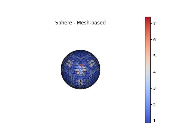
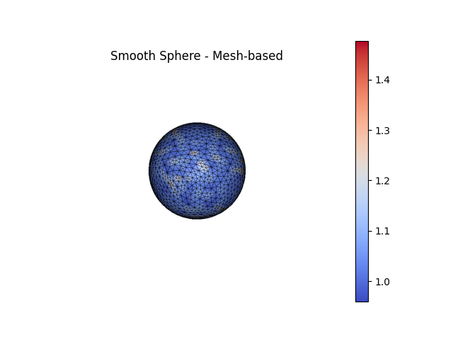
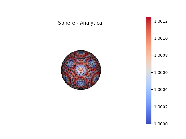
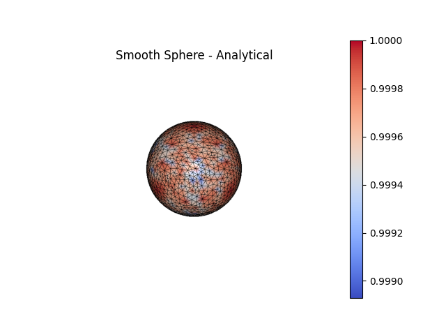
The curvature of two unit spheres is measured with both mesh-based and analytical (implicit function-based) methods. The first sphere is the direct result of marching cubes, which typically contains low quality triangles. The second sphere is a smoothed version of the first where nodes have been redistributed via tangential Laplacian smoothing and moved to lie more closely to the true surface (see SurfaceNodeOptimization()).

import mymesh
from mymesh import curvature, implicit
import numpy as np
import matplotlib.pyplot as plt

Sphere = implicit.SurfaceMesh(implicit.sphere([0,0,0], 1), [-1,1,-1,1,-1,1], 0.1)
Sphere.verbose=False

SmoothSphere = implicit.SurfaceNodeOptimization(Sphere, implicit.sphere([0,0,0], 1), 0.1, iterate=10)
SmoothSphere.verbose=False

Curvature calculation

Curvature can be calculated from the mesh directly or with additional information if the mesh is implicit function- or image-based. Mesh-based methods (e.g. CubicFit()) work best on uniform and high quality meshes but irregular and low quality meshes can introduce significant errors. Function-based curvatures (e.g. AnalyticalCurvature()) are generally much more, accurate, with most of the error arising from interpolation error in the placement of the nodes onto the surface. For a sphere, the Principal Curvatures (\(\kappa_1\), \(\kappa_2\)) are theoretically both equal to the inverse of the radius of the sphere.

k1m_sphere, k2m_sphere = curvature.CubicFit(Sphere.NodeCoords,
                                            Sphere.NodeConn,
                                            Sphere.NodeNeighbors,
                                            Sphere.NodeNormals)
k1m_smooth, k2m_smooth = curvature.CubicFit(SmoothSphere.NodeCoords,
                                            SmoothSphere.NodeConn,
                                            SmoothSphere.NodeNeighbors, SmoothSphere.NodeNormals)

k1a_sphere, k2a_sphere, _, _ = curvature.AnalyticalCurvature(implicit.sphere([0,0,0], 1), Sphere.NodeCoords)
k1a_smooth, k2a_smooth, _, _ = curvature.AnalyticalCurvature(implicit.sphere([0,0,0], 1), SmoothSphere.NodeCoords)

# Plotting:
fig1, ax1 = Sphere.plot(scalars=k1m_sphere, bgcolor='white', show_edges=True, color='coolwarm', show=False, return_fig=True)
ax1.set_title('Sphere - Mesh-based')
fig2, ax2 = SmoothSphere.plot(scalars=k1m_smooth, bgcolor='white', show_edges=True, color='coolwarm', show=False, return_fig=True)
ax2.set_title('Smooth Sphere - Mesh-based')
fig3, ax3 = Sphere.plot(scalars=k1a_sphere, bgcolor='white', show_edges=True, color='coolwarm', show=False, return_fig=True)
ax3.set_title('Sphere - Analytical')
fig4, ax4 = SmoothSphere.plot(scalars=k1a_smooth, bgcolor='white', show_edges=True, color='coolwarm', show=False, return_fig=True)
ax4.set_title('Smooth Sphere - Analytical')

• 
• 
• 
• 

/home/runner/work/mymesh/mymesh/src/mymesh/utils.py:595: RuntimeWarning: invalid value encountered in arccos
  alpha = np.arccos(cosAlpha, out=np.nan*np.ones_like(cosAlpha), where=(cosAlpha>=-1)|(cosAlpha<=1))*Masknan
/home/runner/work/mymesh/mymesh/src/mymesh/curvature.py:501: NumbaPerformanceWarning: np.dot() is faster on contiguous arrays, called on (Array(float64, 2, 'F', False, aligned=True), Array(float64, 2, 'A', False, aligned=True))
  MaxPrincipalDirection = np.dot(np.linalg.inv(R[:3,:3]), np.append(x[:,np.argmax(v)],0)[:,None])[:,0]
/home/runner/work/mymesh/mymesh/src/mymesh/utils.py:595: RuntimeWarning: invalid value encountered in arccos
  alpha = np.arccos(cosAlpha, out=np.nan*np.ones_like(cosAlpha), where=(cosAlpha>=-1)|(cosAlpha<=1))*Masknan
RFBOutputContext()
RFBOutputContext()
RFBOutputContext()
RFBOutputContext()

Error Measurement

To compare how the two methods performed on the two spheres, the root mean square deviation (RMSD) can be calculate to see how much the measured curvatures deviate from the true curvature of 1 mm ^-1.

RMSD_k1m_sphere = np.sqrt(1/len(k1m_sphere) * np.sum((np.array(k1m_sphere) - 1)**2))
RMSD_k1m_smooth = np.sqrt(1/len(k1m_smooth) * np.sum((np.array(k1m_smooth) - 1)**2))

RMSD_k1a_sphere = np.sqrt(1/len(k1a_sphere) * np.sum((np.array(k1a_sphere) - 1)**2))
RMSD_k1a_smooth = np.sqrt(1/len(k1a_smooth) * np.sum((np.array(k1a_smooth) - 1)**2))



width = 0.35
fig, ax = plt.subplots()
ax.bar([-width/2, 1-width/2], [RMSD_k1m_sphere, RMSD_k1a_sphere], width, label='Sphere')
ax.bar([+width/2,1+width/2], [RMSD_k1m_smooth, RMSD_k1a_smooth], width, label='Smooth Sphere')
ax.set_yscale('log')

ax.set_ylabel('Root mean square error')
ax.set_xticks([0,1])
ax.set_xticklabels(['Mesh-based', 'Analytical'])
ax.legend()
ax.set_ylim([10**-4, 10**1])
plt.show()

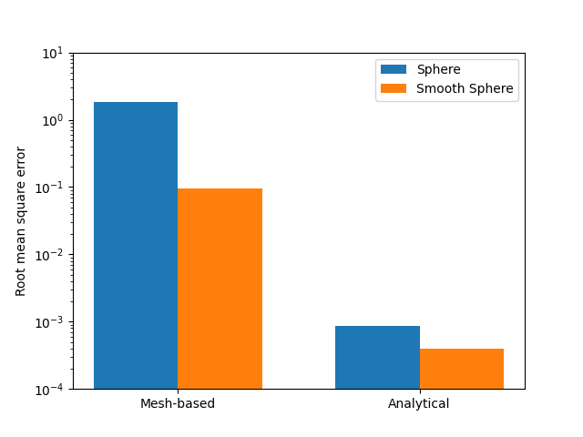
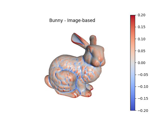
Image-based curvature

For image-based meshes, curvature can be calculated directly from the image and then evaluated at the nodes of the mesh.

# load the CT scan of the Stanford bunny as an example
threshold = 100
scalefactor = 0.5
bunny_img = mymesh.demo_image('bunny', scalefactor=scalefactor)
voxelsize = np.array((0.337891, 0.337891, 0.5))/scalefactor # (mm)

# create a surface mesh of the imaged-object
bunny_surf = mymesh.image.SurfaceMesh(bunny_img, voxelsize, threshold)

# calculate image-based curvatures
sigma = 1 # (voxels) Sets the standard deviation used for calculating derivativess
maxp, minp, mean, gaussian = curvature.ImageCurvature(bunny_img, voxelsize,
                                                     bunny_surf.NodeCoords,
                                                     gaussian_sigma=sigma)
bunny_surf.NodeData['Mean Curvature (Image)'] = mean

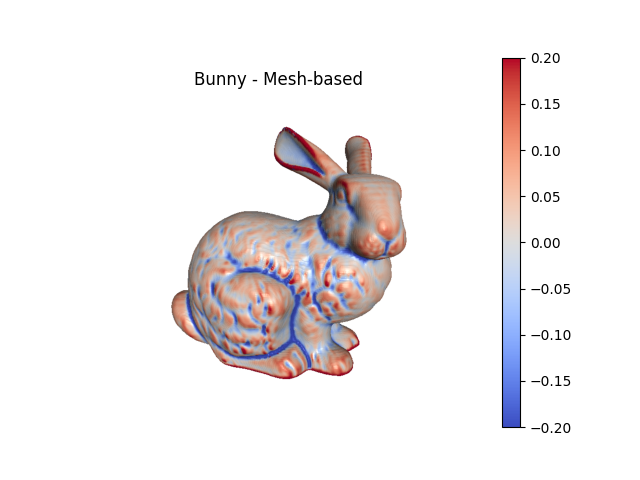
# calculate mesh-based curvatures for comparison (using a 3-ring neighborhood)
mesh_curvatures = bunny_surf.getCurvature(nRings=3)
bunny_surf.NodeData['Mean Curvature (Mesh)'] = mesh_curvatures['Mean Curvature']

# plotting:
fig1, ax1 = bunny_surf.plot(scalars='Mean Curvature (Image)', clim=(-.2,.2),
                             color='coolwarm', show=False, return_fig=True,
                             view='-x-z')
ax1.set_title('Bunny - Image-based')
fig2, ax2 = bunny_surf.plot(scalars='Mean Curvature (Mesh)', clim=(-.2,.2),
                             color='coolwarm', show=False, return_fig=True,
                             view='-x-z')
ax2.set_title('Bunny - Mesh-based')

• 
• 

Calculating surface node normals...
        Identifying surface node element connectivity...Done

        Calculating surface element normals...Done
        Done
RFBOutputContext()

Identifying mesh nodes...Done
        RFBOutputContext()